EEG Classification and Diffusion

Project Overview

In this project, myself and three other UCLA students explored the efficacy of using diffusion to generate EEG signals to train classification. We would like to thank the Graz University of Technology, Austria for allowing us to use their EEG dataset for our project. The dataset can be found here.

Project Goals

The main goal of the project was maximizing the classification accuracy of different movements of a person based on EEG signals. We also wanted to explore the efficacy of using diffusion to generate EEG signals for classification. We also wanted to explore the efficacy of using different variations of CNNs for classification, specificially if a simple CNN would be better than a CNN with an LSTM or Multi-Head Attention layer.

Project Results

We found that using a simple CNN was the best model for classifying EEG signals, achieving a classification test accuracy of 70.4%. We also found that using diffusion to generate EEG signals was not as effective as we hoped for, which we attributed to the small amount of data and the amount of noise in the data. We also found that using a simple CNN was the best model for classifying EEG signals.

Hyperparameter Tuning

Here is a table of the different model architectures that we tested and their respective accuracies, both in total over all subjects and per subject:

Architecture	Test Acc	Sub 1 TA	Sub 2 TA	Sub 3 TA	Sub 4 TA	Sub 5 TA	Sub 6 TA	Sub 7 TA	Sub 8 TA	Sub 9 TA
CNN, No Aug	54.2	46.0	42.0	52.0	64.0	61.7	55.1	64.0	48.0	55.3
CNN, All subs	69.5	62.3	55.4	72.3	71.1	80.5	63.6	74.3	62.6	76.9
CNN Optimized, All subs	70.4	65.0	56.0	72.5	70.5	79.3	63.8	71.5	65.5	78.8
CNN+LSTM, All subs	55.6	42.0	42.0	59.7	59.7	70.5	52.2	59.7	46.5	69.0
CNN+MHA, All subs	62.3	56.0	49.1	63.4	58.9	75.7	66.5	59.4	59.4	67.8
CNN, Sub 1	29.7	36.3	24.6	23.7	35.1	23.4	24.5	32.3	30.3	35.0
CNN+LSTM, Sub 1	21.7	22.4	18.0	28.0	28.0	17.0	20.4	16.0	22.0	25.5
CNN+MHA, Sub 1	33.0	24.3	29.1	34.6	34.0	24.3	34.1	32.9	43.1	41.6

In the above table, CNN Optimized is a CNN with optimized kernel sizes and strides. CNN+LSTM is a CNN with an LSTM layer after the CNN. CNN+MHA is a CNN with a Multi-Head Attention layer after the CNN. All subs means that the model was trained on all subjects. Sub 1 means that the model was trained on subject 1. As we can see, the CNN Optimized model performed the best out of all the models that we tested when trained on all subjects. The CNN+MHA model performed the best when trained on subject 1.

We also found that having a time window of 384 ms was the best time window for classification, with the lowest accuracies happening at 32 ms and 500 ms.

Diffusion

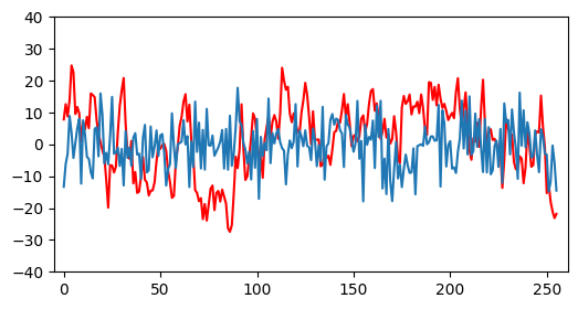
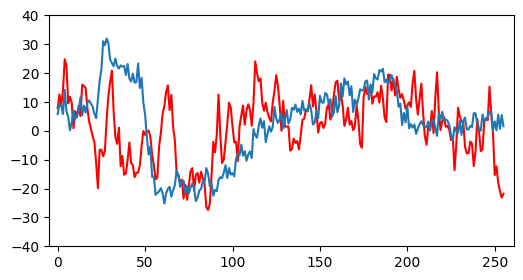
Here is an example of one of the generated EEG signals with an example of a real EEG signal:

The real EEG signal is the red line and the generated EEG signal is the blue line. For this graph, the generated EEG signal recieved random noise as input for the diffusion model. As we can see, the generated EEG signal is very noisy and does not resemble the real EEG signal.

The real EEG signal is the red line and the generated EEG signal is the blue line. For this graph, the generated EEG signal recieved the per-channel average of the EEG signals as input for the diffusion model. As we can see, the generated EEG signal is noisy, but has some structure.

Visually, these signals are varying in quality. The random noise signal is very noisy and does not resemble the real EEG signal. The average signal is less noisy and has some structure, but still has some noise in it. We also validated this finding numerically by training a simple CNN on the generated EEG signals and found that the model was not able to classify the signals well. The best model that was trained on the generated signals achieved a test accuracy of 66.9 with 60% synthetic data and 40% real data.

Project Code

The code for this project can be found on my github. The code will be refactored and cleaned up in the future.